The World Cup: a sporting, cultural, social, political, economic, and above all passionate event. The World Cup is the football world’s greatest focus right now, and of course Algolritmo couldn’t miss the chance to bring a statistical and mathematical perspective on this incredible tournament that takes over the news, our conversations, and our daily routines every four years. Today we present the probability of each national team becoming champion — results first, followed by a more detailed explanation of the model for those who want to dig deeper. In upcoming posts we’ll bring more content, such as a betting pool guide and the most likely knockout-stage matchups, so stay tuned to the blog and remember to follow our Facebook page!
Results:
According to the model developed by Algolritmo, these are the chances of each team winning the World Cup:
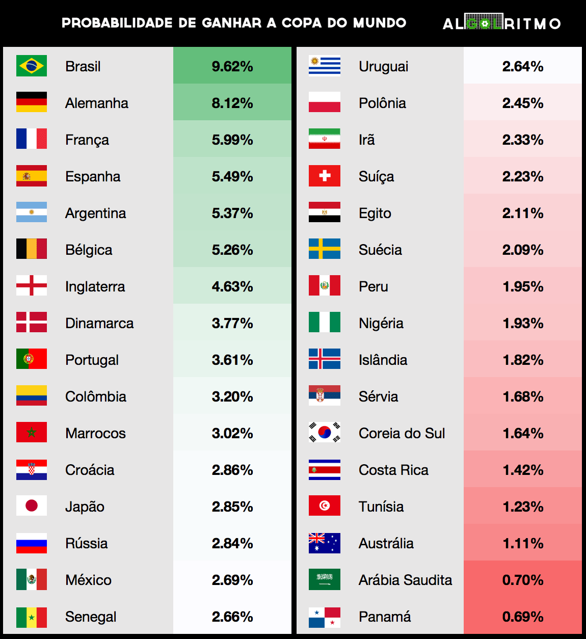
According to our model, the main candidate to win the tournament in Russia is Brazil. The Brazilian squad has improved enormously since the arrival of coach Tite and stands out as one of the favourites to lift the trophy and win the sixth title (“Hexa”). As expected, the other teams with strong chances of winning the World Cup are Germany, France, Spain, Argentina, and Belgium. There is of course a great deal of unpredictability in a short tournament like the World Cup, but it is very unlikely that the champion will come from outside the teams listed above.
What is your prediction for this eagerly awaited World Cup? Are you, like Algolritmo, confident that Brazil will bring home the Hexa? In your opinion, who are the main rivals and possible obstacles?
If you want to understand in more detail how the probabilities above were calculated, here is the model explanation:
Model Assumptions:
- Friendlies carry less importance than official competition matches when assessing a team’s quality.
- Recent matches are more relevant than those played in the more distant past.
- Games against stronger, more traditional opponents are more significant than games against weaker, less established teams. For example, winning 3–0 against Argentina is more impressive than thrashing San Marino 5–0.
- Scoring goals involves randomness, however better teams have greater chances of scoring. To capture the randomness effect, we use the Poisson distribution, as numerous studies have already shown that the number of goals scored by a team follows this type of distribution. (See more in the notes at the end of the text.)
- We will assume that the number of goals scored by a team during a simulated match is decided by rolling a “weighted die”. Each team will have its own die with a different “weight” — that is, each die will have different probabilities for each number of goals. For example, the die rolled by stronger teams (such as Spain) is more likely to land on high values like 4, while the die rolled by weaker teams (such as South Korea) is more likely to land on low values like 1.
The Model:
The idea of the model is to simulate the upcoming World Cup 10,000 times using these weighted dice and analyse the most likely outcomes — a process known as Monte Carlo simulation. To define the weight of the dice rolled by each team in each game, we first need some measure of each team’s offensive and defensive quality.
Generally, the attacking and defensive strength of football teams can be simply calculated and approximated by the average goals scored and conceded over a year. However, for national teams this metric would be quite imprecise for the following reasons:
- National teams play very few times during a year, making the average highly sensitive to any single result.
- A large portion of national team games are friendlies, where the level of competitiveness is lower. Moreover, teams don’t always field their strongest line-ups as many tests are carried out.
- Countries play against very different opponents over a year — some teams face multiple world champions while others play against considerably weaker sides.
With this in mind, the offensive and defensive quality indicators for each team were calculated using data from international matches played over the last 8 years (specifically since 1 August 2010), along with the following variables:
- Number of goals scored in each match.
- Number of goals conceded in each match.
- Time interval (in number of six-month periods) between the match and the start of the 2018 World Cup.
- Match type, i.e. whether the match was a friendly or part of an official competition.
- Strength of the opponent, calculated via Elo rating (an index that assesses team quality).
- Home advantage, whether the team analysed played at home, away, or on a neutral ground.
(For more details on how these different factors were used, see the “Notes” section.)
This made it possible to obtain an offensive and defensive indicator for each team, which can be understood as more accurate, adjusted versions of the average goals scored and average goals conceded. Here are these values for each country:
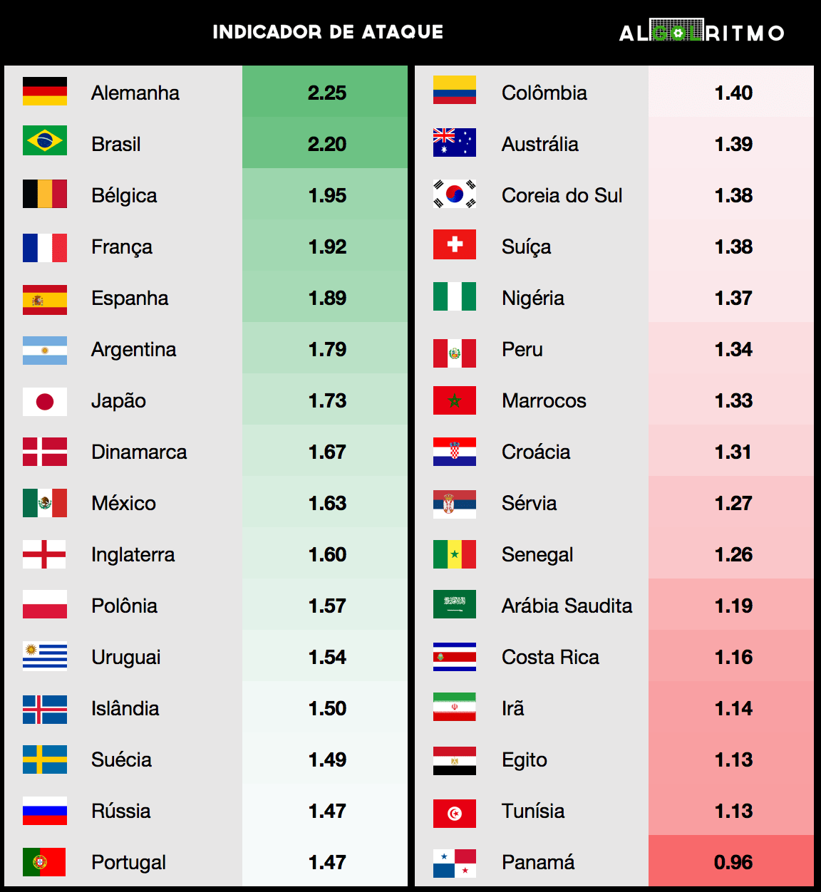
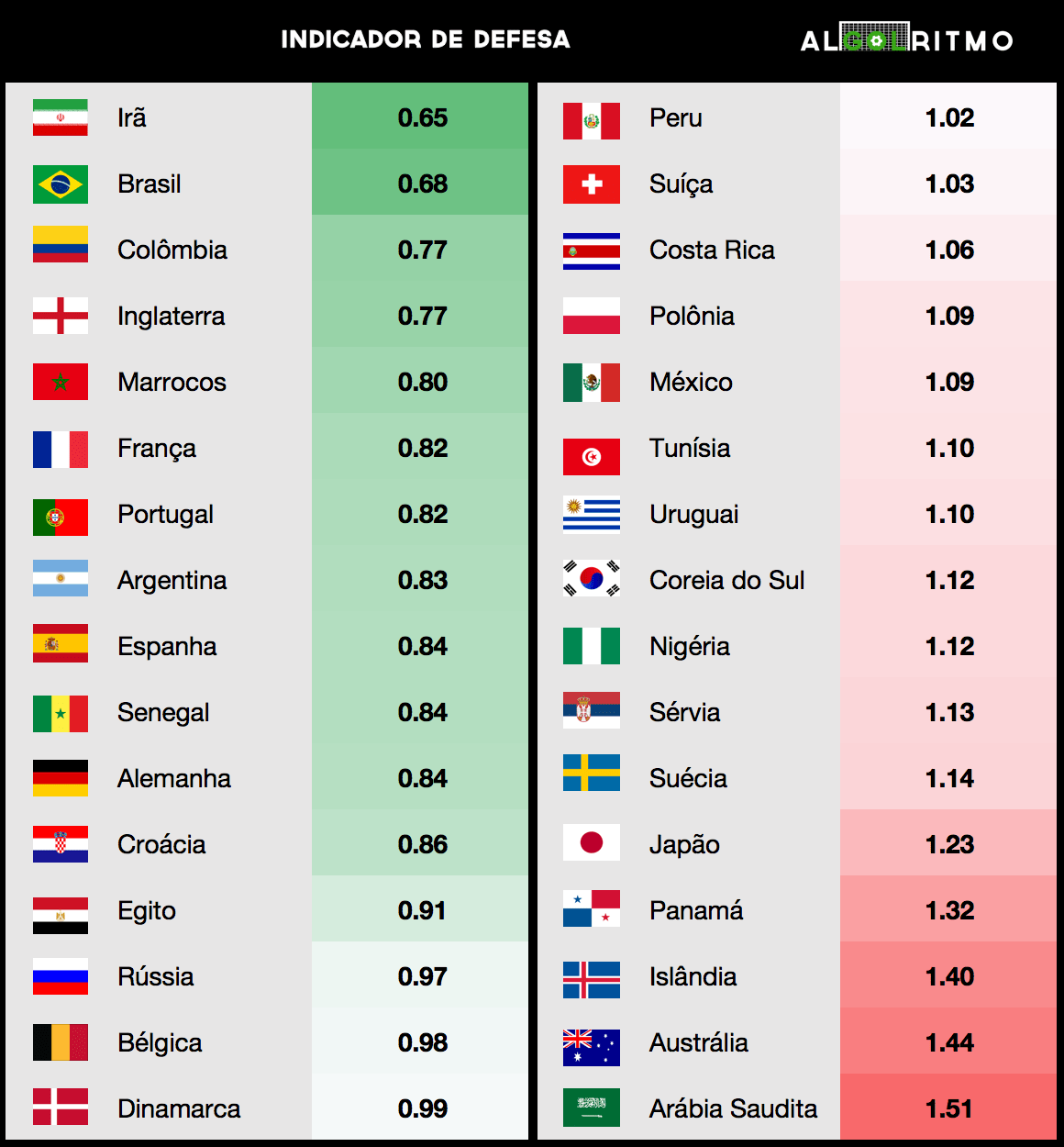
It is of course possible to question some of the values above, which may not seem very intuitive. The most notable is Iran having the best defensive indicator. This happens because Iran genuinely has a defence that is hard to break down for most opponents, often keeping a clean sheet. Even though the model adjusts for the quality of the countries Iran usually faces, the Iranian national team does tend to have a strong defensive instinct — for example at the last World Cup the team put up a tough fight against Argentina and was only defeated by a Messi goal in added time (46th minute of the second half). It is worth noting that despite a certain defensive consistency, the team is extremely unproductive in attack: Iran has the 4th worst offensive indicator among World Cup participants.
To simulate the number of goals scored by a team, a parameter is needed to estimate the “expected average goals” for that team in that matchup. For each game, this is calculated as the average of one team’s offensive indicator and the other team’s defensive indicator. For example, the parameter to simulate the number of goals scored by Russia against Saudi Arabia is: (Russia’s offensive indicator + Saudi Arabia’s defensive indicator) / 2, with numerical values (1.47 + 1.51) / 2 resulting in 1.49. To obtain the parameter to simulate the number of goals scored by Saudi Arabia in that same game, the formula would be: (Saudi Arabia’s offensive indicator + Russia’s defensive indicator) / 2, numerically (1.19 + 0.97) / 2 resulting in 1.08.
Once these results were calculated, I wrote a program in R capable of simulating the upcoming World Cup 10,000 times and analysing the probability of each team winning. The data from these simulations will be used in future posts, so stay tuned to our blog!
Notes:
- For more on the Poisson distribution and its relationship to the number of goals scored, there is a more detailed explanation in this post I wrote about the 2017 Champions League.
- Russia, as the host country, received a bonus of +0.1 and −0.1 on their offensive and defensive indices respectively.
- In calculating the offensive and defensive indices, friendlies were given a weight of 0.5× a regular match.
- To incorporate the time interval effect between the analysed match and the start of the World Cup, I used a weight that decreases exponentially with the following formula (used similarly in the book Mathletics):
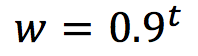
- t = number of six-month periods between the match and the World Cup.
- w = “time weight” of the match.
- Thus, matches that took place in the same six-month period as the World Cup have weight 1, matches from one period earlier have weight 0.9, two periods earlier have weight 0.9 × 0.9, and so on.
- The value of 0.9 is recommended for some sports in the book cited.
- To account for differences between teams, I used the Elo index. This index provides a formula to analyse the probability that a team “does not lose” a game given their ranking points and those of their opponent.
- The weight of each match was (1 – probability of not losing), so more difficult matches carried greater weight.
- If the team played at home, 100 points were added to their Elo index.
- The formula is as follows:
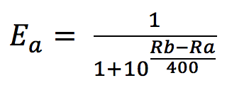
- Ea = probability of team A not losing
- Rb = team B’s Elo points
- Ra = team A’s Elo points